Road detection using segmentation models and albumentations libraries on Keras
In this article, I will show how to write own data generator and how to use albumentations as augmentation library. Along with segmentation_models library, which provides dozens of pretrained heads to Unet and other unet-like architectures. For the full code go to Github. Link to dataset.
-
Original Medium post
Theory
The task of semantic image segmentation is to label each pixel of an image with a corresponding class of what is being represented. For such a task, Unet architecture with different variety of improvements has shown the best result. The core idea behind it just few convolution blocks, which extracts deep and different type of image features, following by so-called deconvolution or upsample blocks, which restore the initial shape of the input image. Besides after each convolution layers, we have some skip-connections, which help the network to remember about initial image and help against fading gradients. For more detailed information you can read the arxiv article or another article.
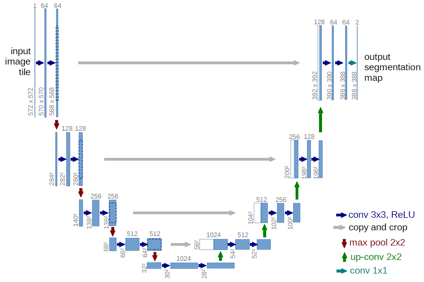 Vanilla U-Net https://arxiv.org/abs/1505.04597
We came for practice, lets go for it.
Dataset—satellite images
For segmentation we don’t need much data to start getting a decent result, even 100 annotated photos will be enough. For now, we will be using Massachusetts Roads Dataset from https://www.cs.toronto.edu/~vmnih/data/, there about 1100+ annotated train images, they even provide validation and test dataset. Unfortunately, there is no download button, so we have to use a script. This script will get the job done (it might take some time to complete).
Lets take a look at image examples:
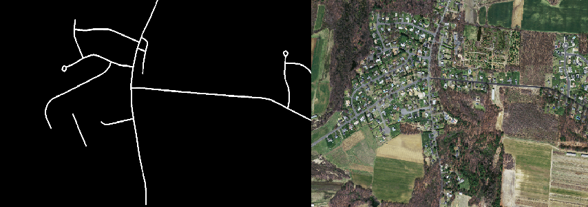 Massachusetts Roads Dataset image and ground truth mask ex.
Annotation and image quality seem to be pretty good, the network should be able to detect roads.
Libraries installation
First of all, you need Keras with TensorFlow to be installed. For Unet construction, we will be using Pavel Yakubovskiy`s library called segmentation_models, for data augmentation albumentation library. I will write more detailed about them later. Both libraries get updated pretty frequently, so I prefer to update them directly from git.
conda install -c conda-forge keras
pip install git+https://github.com/qubvel/efficientnet
pip install git+https://github.com/qubvel/classification_models.git
pip install git+https://github.com/qubvel/segmentation_models
pip install git+https://github.com/albu/albumentations
pip install tta-wrapper
Defining data generator
As a data generator, we will be using our custom generator. It should inherit keras.utils.Sequence and should have defined such methods:
__init__(class initializing)__len__(return lengths of dataset)on_epoch_end(behavior at the end of epochs)__getitem__(generated batch for feeding into a network)
One main advantage of using a custom generator is that you can work with every format data you have and you can do whatever you want — just don’t forget about generating desired output(batch) for keras.
Here we defining __init__ method. The main part of it is setting paths for images (self.image_filenames) and mask names (self.mask_names). Don’t forget to sort them, because for self.image_filenames[i] corresponding mask should be self.mask_names[i].
def __init__(self, root_dir=r'../data/val_test', image_folder='img/', mask_folder='masks/',
             batch_size=1, image_size=768, nb_y_features=1,
             augmentation=None,
             suffle=True):
    self.image_filenames = listdir_fullpath(os.path.join(root_dir, image_folder))
    self.mask_names = listdir_fullpath(os.path.join(root_dir, mask_folder))
    self.batch_size = batch_size
    self.augmentation = augmentation
    self.image_size = image_size
    self.nb_y_features = nb_y_features
    self.suffle = suffle

def listdir_fullpath(d):
    return np.sort([os.path.join(d, f) for f in os.listdir(d)])
Next important thing __getitem__. Usually, we can not store all images in RAM, so every time we generate a new batch of data we should read corresponding images. Below we define the method for training. For that, we create an empty numpy array (np.empty), which will store images and mask. Then we read images by read_image_mask method, apply augmentation into each pair of image and mask. Eventually, we return batch (X, y), which is ready to be fitted into the network.
def __getitem__(self, index):
      data_index_min = int(index*self.batch_size)
      data_index_max = int(min((index+1)*self.batch_size, len(self.image_filenames)))

      indexes = self.image_filenames[data_index_min:data_index_max]
      this_batch_size = len(indexes) # The last batch can be smaller than the others

      X = np.empty((this_batch_size, self.image_size, self.image_size, 3), dtype=np.float32)
      y = np.empty((this_batch_size, self.image_size, self.image_size, self.nb_y_features), dtype=np.uint8)

      for i, sample_index in enumerate(indexes):

          X_sample, y_sample = self.read_image_mask(self.image_filenames[index * self.batch_size + i],
                                                  self.mask_names[index * self.batch_size + i])

          # if augmentation is defined, we assume its a train set
          if self.augmentation is not None:

              # Augmentation code
              augmented = self.augmentation(self.image_size)(image=X_sample, mask=y_sample)
              image_augm = augmented['image']
              mask_augm = augmented['mask'].reshape(self.image_size, self.image_size, self.nb_y_features)
              # divide by 255 to normalize images from 0 to 1
              X[i, ...] = image_augm/255
              y[i, ...] = mask_augm
          else:
              ...
    return X, y
test_generator = DataGeneratorFolder(root_dir = './data/road_segmentation_ideal/training',
                           image_folder = 'input/',
                           mask_folder = 'output/',
                           nb_y_features = 1)

train_generator = DataGeneratorFolder(root_dir = './data/road_segmentation_ideal/training',
                                      image_folder = 'input/',
                                      mask_folder = 'output/',
                                      batch_size=4,
                                      image_size=512,
                                      nb_y_features = 1, augmentation = aug_with_crop)
Data augmentation — albumentations
Data augmentation is a strategy that enables to significantly increase the diversity of data available for training models, without actually collecting new data. It helps to prevent over-fitting and make the model more robust. There are plenty of libraries for such task: imaging, augmentor, solt, built-in methods to keras/pytorch, or you can write your custom augmentation with OpenCV library. But I highly recommend albumentations library. It’s super fast and convenient to use. For usage examples go to the official repository or take a look at example notebooks.
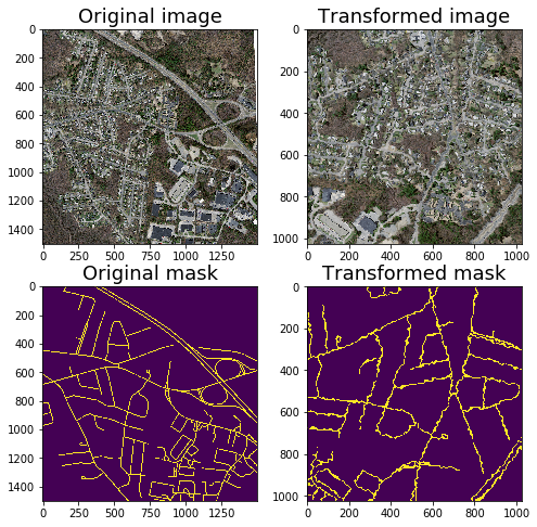
In our task, we will be using basic augmentations such as flips and contrast with non-trivial such ElasticTransform. Example of them you can in the image above.
def aug_with_crop(image_size = 256, crop_prob = 1):
    return Compose([
        RandomCrop(width = image_size, height = image_size, p=crop_prob),
        HorizontalFlip(p=0.5),
        VerticalFlip(p=0.5),
        RandomRotate90(p=0.5),
        Transpose(p=0.5),
        ShiftScaleRotate(shift_limit=0.01, scale_limit=0.04, rotate_limit=0, p=0.25),
        RandomBrightnessContrast(p=0.5),
        RandomGamma(p=0.25),
        IAAEmboss(p=0.25),
        Blur(p=0.01, blur_limit = 3),
        OneOf([
            ElasticTransform(p=0.5, alpha=120, sigma=120 * 0.05, alpha_affine=120 * 0.03),
            GridDistortion(p=0.5),
            OpticalDistortion(p=1, distort_limit=2, shift_limit=0.5)
        ], p=0.8)
    ], p = 1)
After defining the desired augmentation you can easily get your output this:
augmented = aug_with_crop(image_size = 1024)(image=img, mask=mask)
image_aug = augmented['image']
mask_aug = augmented['mask']
Callbacks
We will be using common callbacks:
- ModelCheckpoint — allows you to save weights of the model while training
- ReduceLROnPlateau — reduces training if a validation metric stops to increase
- EarlyStopping — stop training once metric on validation stops to increase several epochs
- TensorBoard — the great way to monitor training progress
from keras.callbacks import ModelCheckpoint, ReduceLROnPlateau, EarlyStopping, TensorBoard

# reduces learning rate on plateau
lr_reducer = ReduceLROnPlateau(factor=0.1,
                               cooldown= 10,
                               patience=10,verbose =1,
                               min_lr=0.1e-5)
# model autosave callbacks
mode_autosave = ModelCheckpoint("./weights/road_crop.efficientnetb0imgsize.h5",
                                monitor='val_iou_score',
                                mode='max', save_best_only=True, verbose=1, period=10)

# stop learining as metric on validatopn stop increasing
early_stopping = EarlyStopping(patience=10, verbose=1, mode = 'auto')

# tensorboard for monitoring logs
tensorboard = TensorBoard(log_dir='./logs/tenboard', histogram_freq=0,
                          write_graph=True, write_images=False)

callbacks = [mode_autosave, lr_reducer, tensorboard, early_stopping]
Training
As the model, we will be using Unet. The easiest way to use it just get from segmentation_models library.
- backbone_name: name of classification model for using as an encoder. EfficientNet currently is state-of-the-art in the classification model, so let us try it. While it should give faster inference and has less training params, it consumes more GPU memory than well-known resnet models. There are many other options to try
- encoder_weights — using imagenet weights speeds up training
- encoder_freeze: if True set all layers of an encoder (backbone model) as non-trainable. It might be useful firstly to freeze and train model and then unfreeze
- decoder_filters — you can specify numbers of decoder block. In some cases, a heavier encoder with simplified decoder might be useful.
After initializing Unet model, you should compile it. Also, we set IOU ( intersection over union) as metric we will to monitor and bce_jaccard_loss (binary cross-entropy plus jaccard loss) as the loss we will optimize. I gave links, so won’t go here for further detail for them.
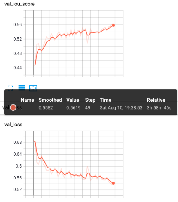 Tensorboard logs
After starting training you can for watching tensorboard logs. As we can see model train pretty well, even after 50 epoch we didn’t reach global/local optima.
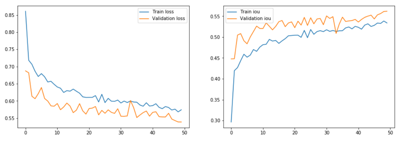 Loss and IOU metric history
Inference
So we have 0.558 IOU on validation, but every pixel prediction higher than 0 we count as a mask. By picking the appropriate threshold we can further increase our result by 0.039 (7%).
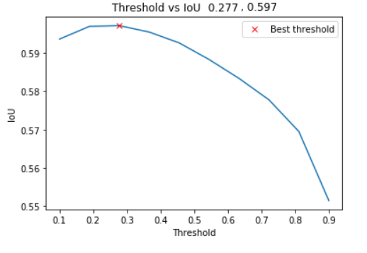 Validation threshold adjusting
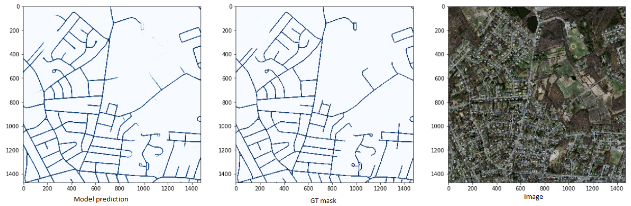
Metrics are quite interesting for sure, but a much more insightful model prediction. From the images below we see that our network caught up the task pretty good, which is great. For the inference code and for calculating metrics you can read full code.
References
@phdthesis{MnihThesis,
    author = {Volodymyr Mnih},
    title = {Machine Learning for Aerial Image Labeling},
    school = {University of Toronto},
    year = {2013}
}