GANs for tabular data
We well know GANs for success in the realistic image generation. However, they can be applied in tabular data generation. We will review and examine some recent papers about tabular GANs in action.
-
Originally posted on Medium.
-
Github repo
What is GAN
“GAN composes of two deep networks: the generator and the discriminator” [1]. Both of them simultaneously trained. Generally, the model structure and training process presented this way:
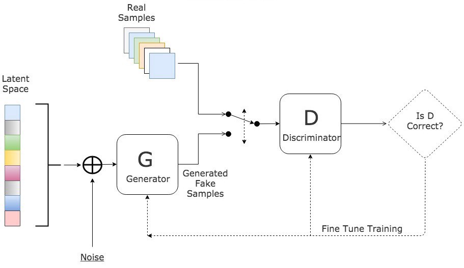 GAN training pipeline. By Jonathan Hui — What is Generative Adversarial Networks GAN? [1]
The task for the generator is to generate samples, which won’t be distinguished from real samples by the discriminator. I won’t give much detail here, but if you would like to dive into them, you can read the medium post and the original paper by Ian J. Goodfellow. Recent architectures such as StyleGAN 2 can produce outstanding photo-realistic images.
 Hand-picked examples of human faces generated by StyleGAN 2, Source arXiv:1912.04958v2 [7]
Problems
While face generation seems to be not a problem anymore, there are plenty of issues we need to resolve:
- Training speed. For training StyleGAN 2 you need 1 week and DGX-1 (8x NVIDIA Tesla V100).
- Image quality in specific domains. The state-of-the-art network still fails on other tasks.
 Hand-picked examples of cars and cats generated by StyleGAN 2, Source arXiv:1912.04958v2 [7]
Tabular GANs
Even cats and dogs generation seem heavy tasks for GANs because of not trivial data distribution and high object type variety. Besides such domains, the image background becomes important, which GANs usually fail to generate. Therefore, I’ve been wondering what GANs can achieve in tabular data. Unfortunately, there aren’t many articles. The next two articles appear to be the most promising.
TGAN: Synthesizing Tabular Data using Generative Adversarial Networks arXiv:1811.11264v1 [3]
First, they raise several problems, why generating tabular data has own challenges: the various data types (int, decimals, categories, time, text) different shapes of distribution ( multi-modal, long tail, Non-Gaussian…) sparse one-hot-encoded vectors and highly imbalanced categorical columns.
Task formalizing
Let us say table T contains n_c continuous variables and n_d discrete(categorical) variables, and each row is C vector. These variables have an unknown joint distribution P. Each row is independently sampled from P. The object is to train a generative model M. M should generate new a synthetic table T_synth with the distribution similar to P. A machine learning model learned on T_synth should achieve a similar accuracy on a real test table T_test, as would a model trained on T.
Preprocessing numerical variables
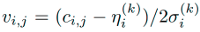
“Neural networks can effectively generate values with a distribution centered over (−1, 1) using tanh” [3]. However, they show that nets fail to generate suitable data with multi-modal data. Thus they cluster a numerical variable by using and training a Gaussian Mixture Model (GMM) with m (m=5) components for each of C.
 Normalizing using GMM using mean and standard deviation. Source arXiv:1811.11264v1 [3]
Finally, GMM is used to normalize C to get V. Besides, they compute the probability of C coming from each of the m Gaussian distribution as a vector U.
Preprocessing categorical variables
Due to usually low cardinality, they found the probability distribution can be generated directly using softmax. But it necessary to convert categorical variables to one-hot-encoding representation with noise to binary variables After prepossessing, they convert T with n_c + n_d columns to V, U, D vectors. This vector is the output of the generator and the input for the discriminator in GAN. “GAN does not have access to GMM parameters” [3].
Generator
They generate a numerical variable in 2 steps. First, generate the value scalar V, then generate the cluster vector U eventually applying tanh. Categorical features generated as a probability distribution over all possible labels with softmax. To generate the desired row LSTM with attention mechanism is used. Input for LSTM in each step is random variable z, weighted context vector with previous hidden and embedding vector.
Discriminator
Multi-Layer Perceptron (MLP) with LeakyReLU and BatchNorm is used. The first layer used concatenated vectors (V, U, D) among with mini-batch diversity with feature vector from LSTM. The loss function is the KL divergence term of input variables with the sum ordinal log loss function.
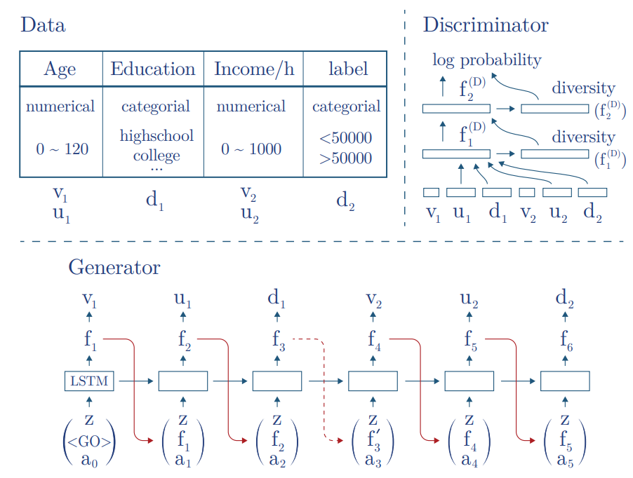 Example of using TGAN to generate a simple census table. The generator generates T features one be one. The discriminator concatenates all features together. Then it uses Multi-Layer Perceptron (MLP) with LeakyReLU to distinguish real and fake data. Source arXiv:1811.11264v1 [3]
Results
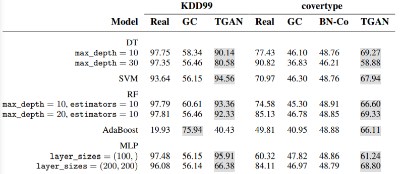 Accuracy of machine learning models trained on the real and synthetic training set. (BN — Bayesian networks, Gaussian Copula). Source arXiv:1811.11264v1 [3]
They evaluate the model on two datasets KDD99 and covertype. For some reason, they used weak models without boosting (xgboost, etc). Anyway, TGAN performs reasonably well and robust, outperforming bayesian networks. The average performance gap between real data and synthetic data is 5.7%.
Modeling Tabular Data using Conditional GAN (CTGAN) arXiv:1907.00503v2 [4]
The key improvements over previous TGAN are applying the mode-specific normalization to overcome the non-Gaussian and multimodal distribution. Then a conditional generator and training-by-sampling to deal with the imbalanced discrete columns.
Task formalizing
The initial data remains the same as it was in TGAN. However, they solve different problems.
- Likelihood of fitness. Do columns in T_syn follow the same joint distribution as T_train
- Machine learning efficacy. When training model to predict one column using other columns as features, can such model learned from T_syn achieve similar performance on T_test, as a model learned on T_train
Preprocessing
Preprocessing for discrete columns keeps the same. For continuous variables, a variational Gaussian mixture model (VGM) is used. It first estimates the number of modes m and then fits a Gaussian mixture. After we normalize initial vector C almost the same as it was in TGAN, but the value is normalized within each mode. Mode is represented as one-hot vector betta ([0, 0, .., 1, 0]). Alpha is the normalized value of C.
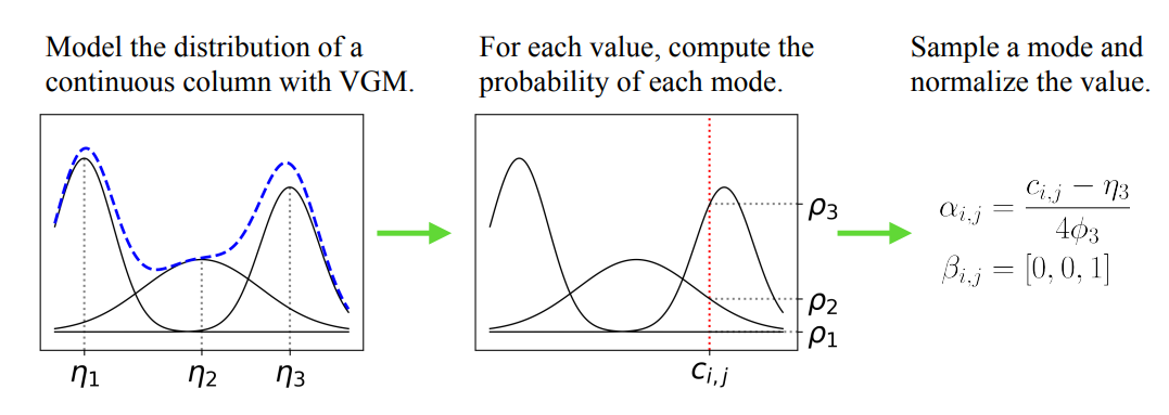 An example of mode-specific normalization. Source arXiv:1907.00503v2 [4]
As a result, we get our initial row represented as the concatenation of one-hot’ ed discrete columns with representation discussed above of continues variables:
 Preprocessed row. Source arXiv:1907.00503v2 [4]
Training
“The final solution consists of three key elements, namely: the conditional vector, the generator loss, and the training-by-sampling method” [4].
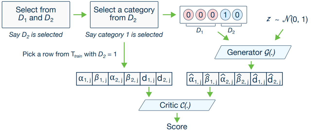 CTGAN model. The conditional generator can generate synthetic rows conditioned on one of the discrete columns. With training-by-sampling, the cond and training data are sampled according to the log-frequency of each category, thus CTGAN can evenly explore all possible discrete values. Source arXiv:1907.00503v2 [4]
Conditional vector
Represents concatenated one-hot vectors of all discrete columns but with the specification of only one category, which was selected. “For instance, for two discrete columns, D1 = {1, 2, 3} and D2 = {1, 2}, the condition (D2 = 1) is expressed by the mask vectors m1 = [0, 0, 0] and m2 = [1, 0]; so cond = [0, 0, 0, 1, 0]” [4].
Generator loss
“During training, the conditional generator is free to produce any set of one-hot discrete vectors” [4]. But they enforce the conditional generator to produce d_i (generated discrete one-hot column)= m_i (mask vector) is to penalize its loss by adding the cross-entropy between them, averaged over all the instances of the batch.
Training-by-sampling
“Specifically, the goal is to resample efficiently in a way that all the categories from discrete attributes are sampled evenly during the training process, as a result, to get real data distribution during the test” [4]. In another word, the output produced by the conditional generator must be assessed by the critic, which estimates the distance between the learned conditional distribution P_G(row|cond) and the conditional distribution on real data P(row|cond). “The sampling of real training data and the construction of cond vector should comply to help critics estimate the distance” [4]. Properly sample the cond vector and training data can help the model evenly explore all possible values in discrete columns. The model structure is given below, as opposite to TGAN, there is no LSTM layer. Trained with WGAN loss with gradient penalty.
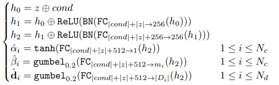 Generator. Source arXiv:1907.00503v2 [4]
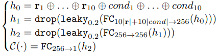 Discriminator. Source arXiv:1907.00503v2 [4]
Also, they propose a model based on Variational autoencoder (VAE), but it out of the scope of this article.
Results
Proposed network CTGAN and TVAE outperform other methods. As they say, TVAE outperforms CTGAN in several cases, but GANs do have several favorable attributes. The generator in GANs does not have access to real data during the entire training process, unlike TVAE.
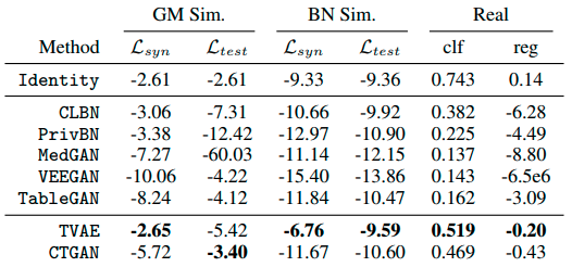 Benchmark results over three sets of experiments, namely Gaussian mixture simulated data (GM Sim.), Bayesian network simulated data (BN Sim.), and real data. They report the average of each metric. For real datasets (f1, etc). Source arXiv:1907.00503v2 [4]
Besides, they published source code on GitHub, which with slight modification will be used further in the article.
Applying CTGAN to generating data for increasing train (semi-supervised)
This is a kind of vanilla dream for me to be examined. After brief familiarization with recent developments in GAN, I’ve been thinking about how to apply it to something that I solve on the work daily. So here is my idea.
Task formalization
Let say we have T_train and T_test (train and test set respectively). We need to train the model on T_train and make predictions on T_test. However, we will increase the train by generating new data by GAN, somehow similar to T_test, without using ground truth labels of it.
Experiment design
Let say we have T_train and T_test (train and test set respectively). The size of T_train is smaller and might have different data distribution. First of all, we train CTGAN on T_train with ground truth labels (step 1), then generate additional data T_synth (step 2). Secondly, we train boosting in an adversarial way on concatenated T_train and T_synth (target set to 0) with T_test (target set to 1) (steps 3 & 4). The goal is to apply newly trained adversarial boosting to obtain rows more like T_test. Note — original ground truth labels aren’t used for adversarial training. As a result, we take top rows from T_train and T_synth sorted by correspondence to T_test (steps 5 & 6). Finally, rain new boosting on them and check results on T_test.
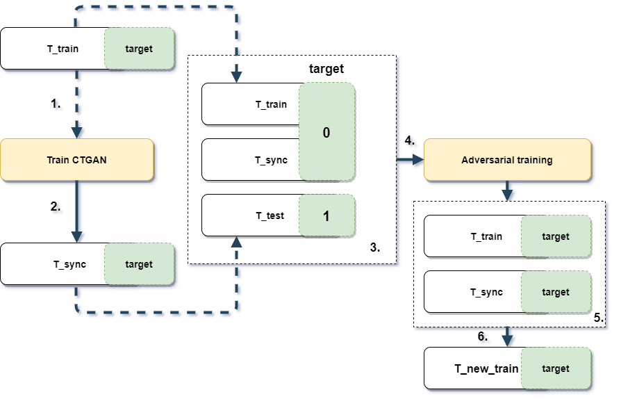 Experiment design and workflow
Of course for the benchmark purposes we will test ordinal training without these tricks and another original pipeline but without CTGAN (in step 3 we won’t use T_sync).
Code
Experiment code and results released as Github repo here. Pipeline and data preparation was based on Benchmarking Categorical Encoders’ article and its repo. We will follow almost the same pipeline, but for speed, only Single validation and Catboost encoder was chosen. Due to the lack of GPU memory, some of the datasets were skipped.
Datasets
All datasets came from different domains. They have a different number of observations, several categorical and numerical features. The aim of all datasets is a binary classification. Preprocessing of datasets was simple: removed all time-based columns from datasets. The remaining columns were either categorical or numerical. In addition, while training results were sampled T_train — 5%, 10%, 25%, 50%, 75%
| Name | Total points | Train points | Test points | Number of features | Number of categorical features | Short description |
|---|---|---|---|---|---|---|
| Telecom | 7.0k | 4.2k | 2.8k | 20 | 16 | Churn prediction for telecom data |
| Adult | 48.8k | 29.3k | 19.5k | 15 | 8 | Predict if persons’ income is bigger 50k |
| Employee | 32.7k | 19.6k | 13.1k | 10 | 9 | Predict an employee’s access needs, given his/her job role |
| Credit | 307.5k | 184.5k | 123k | 121 | 18 | Loan repayment |
| Mortgages | 45.6k | 27.4k | 18.2k | 20 | 9 | Predict if house mortgage is founded |
| Taxi | 892.5k | 535.5k | 357k | 8 | 5 | Predict the probability of an offer being accepted by a certain driver |
| Poverty_A | 37.6k | 22.5k | 15.0k | 41 | 38 | Predict whether or not a given household for a given country is poor or not |
Datasets properties
Results
From the first sight of view and in terms of metric and stability (std), GAN shows the worse results. However, sampling the initial train and then applying adversarial training we could obtain the best metric results and stability (sample_original). To determine the best sampling strategy, ROC AUC scores of each dataset were scaled (min-max scale) and then averaged among the dataset.
Results
To determine the best validation strategy, I compared the top score of each dataset for each type of validation.
Table 1.2 Different sampling results across the dataset, higher is better (100% - maximum per dataset ROC AUC)
| dataset_name | None | gan | sample_original |
|---|---|---|---|
| credit | 0.997 | 0.998 | 0.997 |
| employee | 0.986 | 0.966 | 0.972 |
| mortgages | 0.984 | 0.964 | 0.988 |
| poverty_A | 0.937 | 0.950 | 0.933 |
| taxi | 0.966 | 0.938 | 0.987 |
| adult | 0.995 | 0.967 | 0.998 |
| telecom | 0.995 | 0.868 | 0.992 |
Table 1.3 Different sampling results, higher is better for a mean (ROC AUC), lower is better for std (100% - maximum per dataset ROC AUC)
| sample_type | mean | std |
|---|---|---|
| None | 0.980 | 0.036 |
| gan | 0.969 | 0.06 |
| sample_original | 0.981 | 0.032 |
We can see that GAN outperformed other sampling types in 2 datasets. Whereas sampling from original outperformed other methods in 3 of 7 datasets. Of course, there isn’t much difference. but these types of sampling might be an option. Of course, there isn’t much difference. but these types of sampling might be an option.
Table 1.4 same_target_prop is equal 1 then the target rate for train and test are different no more than 5%. Higher is better.
| sample_type | same_target_prop | prop_test_score |
|---|---|---|
| None | 0 | 0.964 |
| None | 1 | 0.985 |
| gan | 0 | 0.966 |
| gan | 1 | 0.945 |
| sample_original | 0 | 0.973 |
| sample_original | 1 | 0.984 |
Let’s define same_target_prop is equal 1 then the target rate for train and test is different no more than 5%. So then we have almost the same target rate in train and test None and sample_original better. However, gan is starting performing noticeably better than target distribution changes.
same_target_prop is equal 1 then the target rate for train and test are different only by 5%
References
[1] Jonathan Hui. GAN — What is Generative Adversarial Networks GAN? (2018), medium article [2] Ian J. Goodfellow, Jean Pouget-Abadie, Mehdi Mirza, Bing Xu, David Warde-Farley, Sherjil Ozair, Aaron Courville, Yoshua Bengio. Generative Adversarial Networks (2014). arXiv:1406.2661 [3] Lei Xu LIDS, Kalyan Veeramachaneni. Synthesizing Tabular Data using Generative Adversarial Networks (2018). arXiv:1811.11264v1 [cs.LG] [4] Lei Xu, Maria Skoularidou, Alfredo Cuesta-Infante, Kalyan Veeramachaneni. Modeling Tabular Data using Conditional GAN (2019). arXiv:1907.00503v2 [cs.LG] [5] Denis Vorotyntsev. Benchmarking Categorical Encoders (2019). Medium post [6] Insaf Ashrapov. GAN-for-tabular-data (2020). Github repository. [7] Tero Karras, Samuli Laine, Miika Aittala, Janne Hellsten, Jaakko Lehtinen, Timo Aila. Analyzing and Improving the Image Quality of StyleGAN (2019) arXiv:1912.04958v2 [cs.CV]