Graph classification by computer vision
Graph analysis nowadays becomes more popular, but how does it perform compared to the computer vision approach? We will show while the training speed of computer vision models is much slower, they perform considerably well compared to graph theory.
Graph analysis
In general, graph theory represents pairwise relationships between objects. We won’t leave much detail here, but you may consider its some kind of network below:
 Network. Photo by Alina Grubnyak on Unsplash
The main point we need to know here, it is that by connecting objects with edges we may visualize graphs. Then we will be able to use classic computer vision models. Unfortunately, we may lose some initial information. For example, the graph may contain different types of objects, connection, maybe impossible to visualize it in 2D.
Libraries
There are plenty of libraries you look at if you willing to start working with them:
- networkx — classical algorithms, visualizations
- pytorch_geometric — SOTA algorithms graph, a framework on top of pytorch
- graph-tool — classical algorithms, visualizations
- scikit-network — classical algorithms, sklearn like API
- TensorFlow Graphics — SOTA algorithms graph, a framework on top of Tensorflow
They are all aimed at their own specific role. This is why it depends on your task which one to use.
Theory
This article aimed more at practical usage this why for the theory I will leave some only some links:
- Hands-on Graph Neural Networks with PyTorch & PyTorch Geometric
- CS224W: Machine Learning with Graphs
- Graph classification will be based on Graph Convolutional Networks (GCN), arxiv link
Model architecture
We will be using as baseline following architecture:
* GCNConv - 6 blocks
* JumpingKnowledge for aggregation sconvolutions
* global_add_pool with relu
* Final layer is softmax
class SimpleGNN(torch.nn.Module):
    """Original from http://pages.di.unipi.it/citraro/files/slides/Landolfi_tutorial.pdf"""
    def __init__(self, dataset, hidden=64, layers=6):
        super(SimpleGNN, self).__init__()
        self.dataset = dataset
        self.convs = torch.nn.ModuleList()
        self.convs.append(GCNConv(in_channels=dataset.num_node_features,
                                  out_channels=hidden))

        for _ in range(1, layers):
            self.convs.append(GCNConv(in_channels=hidden, out_channels=hidden))

        self.jk = JumpingKnowledge(mode="cat")
        self.jk_lin = torch.nn.Linear(
            in_features=hidden*layers, out_features=hidden)
        self.lin_1 = torch.nn.Linear(in_features=hidden, out_features=hidden)
        self.lin_2 = torch.nn.Linear(
            in_features=hidden, out_features=dataset.num_classes)

    def forward(self, index):
        data = Batch.from_data_list(self.dataset[index])
        x = data.x
        xs = []
        for conv in self.convs:
            x = F.relu(conv(x=x, edge_index=data.edge_index))
            xs.append(x)

        x = self.jk(xs)
        x = F.relu(self.jk_lin(x))
        x = global_add_pool(x, batch=data.batch)
        x = F.relu(self.lin_1(x))
        x = F.softmax(self.lin_2(x), dim=-1)
        return x
The code link is based on this tutorial.
Computer vision
All the required theory and technical skills you will get by following this article: Guide how to learn and master computer vision in 2020 Besides, you should be familiar with the next topics:
- EfficientNet https://arxiv.org/abs/1905.11946
- Focal Loss https://arxiv.org/abs/1708.02002
- albumentations — augmentation library
- pytorch-lightning — pytorch framework
Model architecture
We will be using the following model without any hyper-parameter tuning::
- efficientnet_b2b as encoder
- FocalLoss and average precision as early stopping criteria
- TTA with flip left right and up down
- Augmentation with albumentation
- Pytorch-lightning as training model framework
- 4 Folds Assembling
- mixup The code link.
Experiment
Data
We will predict the activity (against COVID?) of different molecules. Dataset sample:
smiles, activity
OC=1C=CC=CC1CNC2=NC=3C=CC=CC3N2, 1
CC(=O)NCCC1=CNC=2C=CC(F)=CC12, 1
O=C([C@@H]1[C@H](C2=CSC=C2)CCC1)N, 1
To generate images for the computer vision approach we first convert the graph to the networkx format and then get the desired images by calling draw_kamada_kawai function:
""" Full code link
https://github.com/Diyago/Graph-clasification-by-computer-vision/blob/main/generate_images.py"""
if __name__ == "__main__":
    ohd = transforms.OneHotDegree(max_degree=4)
    covid = COVID(root='./data/COVID/', transform=ohd)
    for graph in torch.arange(len(covid)).long():
        G = utils.to_networkx(covid[int(graph)])
        a = nx.draw_kamada_kawai(G)
        plt.savefig("./train/id_{}_y_{}.jpg".format(int(graph),
                                                    covid.data.y[int(graph)]), format="jpg")
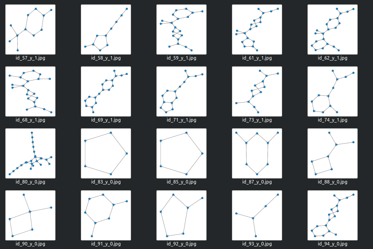 Different molecules visualization will be used for the computer vision approach. Image by Insaf Ashrapov
Link to the dataset.
Experiment results
TEST metrics
### Computer vision
* ROC AUC 0.697
* MAP 0.183

### Graph method
* ROC AUC 0.702
* MAP 0.199
As you can result practically similar. The graph method gets a bit higher results. Besides, it takes only 1 minute to train GNN and 30 minutes for CNN. I have to say: this is mostly just a proof-of-concept project with many simplifications. In other words, you may visualize graphs and train well-known computer vision models instead of fancy-new GNN.
References
- Github repo with all code link by Insaf Ashrapov
- GNN tutorial http://pages.di.unipi.it/citraro/files/slides/Landolfi_tutorial.pdf